Learn how to create an Excel interactive chart with dynamic array. Technically, is an example of How do I create a dynamic bar chart in Excel Or How do you make a dynamic bar chart? This tip and tricks also works for question like What are dynamic charts that update automatically in excel. And how do I create a dynamic range in Excel? And...
Verified link by Valmet Tissue Converting Solutions
How To Create An Excel Interactive Chart With Dynamic Arrays - Excel Tips And Tricks Information Center
Get comprehensive updates, key reports, and detailed insights compiled from verified editorial sources.
Introduction of How To Create An Excel Interactive Chart With Dynamic Arrays - Excel Tips And Tricks

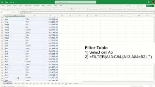
Learn how to create an Excel interactive chart with dynamic array. Technically, is an example of How do I create a dynamic bar chart in Excel Or How do you make a dynamic bar chart? This tip and tricks also works for question like What are dynamic charts that update automatically in excel. And how do I create a dynamic range in Excel? And finally answers to question on how to make an Excel dynamic chart & keep updates consistent? Excel is a powerful tool for data analysis and visualization, and one of its standout features is the ability to create interactive charts. Interactive charts allow users to explore and analyze data dynamically, providing a more engaging and flexible experience. In this article, we will focus on creating an interactive chart with dynamic arrays in Excel. Before we delve into the specifics of creating dynamic charts, let's first understand what dynamic arrays are. Dynamic arrays are a new feature introduced in Excel 365 and Excel 2021 that allow you to work with arrays of values, such as formulas or functions, that can automatically spill into multiple cells. This functionality is particularly useful when dealing with large datasets or when you need to perform calculations across multiple cells simultaneously. Create Month List 1) Select cell B2 2) Data ~ Data Validation 3) Set Allow to List 4) Source as =$A$16:$A$87 5) Apply Filter Table 1) Select cell A5 2) =FILTER(A13:C84,(A13:A84=B2),"") Draw Bar Chart 1) Highlight filtered table (console and sales) 2) Insert ~ Clustered Bar Chart 3) Select x-axis and delete it 4) Right-click on the bar chart, Format 5) Disable Legend Remove Title Horizontal Axis, Uncheck Display axis Series 1, enable Data Labels Fill to Red Label position Center 6) Position the chart to cover Filter Table
Core Information
Explore the main sources for How To Create An Excel Interactive Chart With Dynamic Arrays - Excel Tips And Tricks.
Latest News
Stay updated on How To Create An Excel Interactive Chart With Dynamic Arrays - Excel Tips And Tricks's latest milestones.
Featured Video Reports & Highlights
Below is a handpicked selection of video coverage, expert reports, and highlights regarding How To Create An Excel Interactive Chart With Dynamic Arrays - Excel Tips And Tricks from verified contributors.
How to Create an Excel Interactive Chart with Dynamic Arrays - Excel Tips and Tricks
Detailed Analysis
Data is compiled from public records and verified media reports.
Last Updated: May 23, 2026
Conclusion
For 2026, How To Create An Excel Interactive Chart With Dynamic Arrays - Excel Tips And Tricks remains one of the most searched-for profiles. Check back for the latest updates.
Disclaimer:
